Tabular analysis

Thus far, we’ve read the data files as output by the National Water Model, which are provided as hourly snapshots in NetCDF format (or slight transformations of them, like via Kerchunk index files or conversion to Zarr).

A subset of the data (we’ll look at reservoir data) are distributed as NetCDF files but are fundamentally tabular. As an exercise, I converted some reservoir data to a geoparquet dataset. Parquet is a nice, high-performance dataset for tabular data. Geoparquet is like regular parquet, only with some extra geospatial metadata.

import dask.dataframe as dd
import dask_geopandas
import geopandas

This is a pretty large dataset, partitioned across many individual parquet files, so we’ll load it up with dask.dataframe / dask-geopandas.

df = dd.read_parquet(
    "az://ciroh/short-range-reservoir.parquet/",
    storage_options={"account_name": "noaanwm"},
    calculate_divisions=True,
)
geometry = df.geometry.map_partitions(
    geopandas.GeoSeries.from_wkb,
    meta=geopandas.GeoSeries([], name="geometry"),
    crs="epsg:4326",
)

gdf = dask_geopandas.from_dask_dataframe(df, geometry=geometry)
gdf

Dask-GeoPandas GeoDataFrame Structure:

	feature_id	geometry	reservoir_type	water_sfc_elev	inflow	outflow
npartitions=21
2021-08-26 01:00:00	int32	geometry	category[unknown]	float32	float64	float64
2021-09-01 01:00:00	...	...	...	...	...	...
...	...	...	...	...	...	...
2023-04-01 01:00:00	...	...	...	...	...	...
2023-04-18 23:00:00	...	...	...	...	...	...

Dask Name: GeoDataFrame, 5 graph layers

This data structure shows our 6 columns and their data types.

The output also shows that we have 21 partitions (or individual parquet files). I partitioned the data by month, so we can quickly look up a subset of the data.

w = gdf.loc["2022-07-01":"2022-07-08"]
w.head()

	feature_id	geometry	reservoir_type	water_sfc_elev	inflow	outflow
time
2022-07-01	491	POINT (-68.37904 46.18327)	1	206.158081	0.33	0.55
2022-07-01	531	POINT (-68.45489 46.16116)	1	247.600632	0.03	0.31
2022-07-01	747	POINT (-68.06499 46.03409)	1	190.322128	0.02	0.10
2022-07-01	759	POINT (-68.16213 46.02238)	1	165.124863	0.00	0.17
2022-07-01	1581	POINT (-67.93720 45.64844)	1	130.030273	0.48	0.55

We can do dataframe-style computations, like grouping by feature ID and getting some summary statistics for the inflow variable.

%%time
inflow = (
    df.groupby("feature_id")
    .inflow.agg(["mean", "min", "max", "std", "count"])
    .compute()
)
inflow.head()

CPU times: user 7.45 s, sys: 2.05 s, total: 9.51 s
Wall time: 3.77 s

	mean	min	max	std	count
feature_id
491	0.794296	0.07	15.20	1.006294	13236
531	0.342121	0.00	18.43	0.746961	13236
747	0.416411	0.01	14.90	0.815884	13236
759	0.000389	0.00	0.13	0.004175	13236
1581	1.271340	0.37	5.22	1.113017	13236

Let’s find the feature_id with the largest change in water elevation in the first month.

xs = gdf.get_partition(0).compute()
change = (
    xs.groupby("feature_id")
    .water_sfc_elev.agg(["min", "max"])
    .diff(axis="columns")["max"]
)
feature_id = change.idxmax()
feature_id

22472505

We can get the geometry for that feature ID.

from ipyleaflet import Map, CircleMarker


geometry = xs[xs.feature_id == feature_id].iloc[0].geometry
y, x = geometry.y, geometry.x

m = Map(center=(y, x), zoom=15)
m.add(CircleMarker(location=(y, x)))
m.scroll_wheel_zoom = True
m

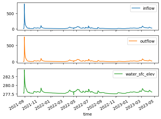
Now let’s examine the timeseries for that particular feature_id.

With dask.dataframe.read_parquet and pyarrow, we can supply a filters argument to efficiently filter the data based on the values, to avoid loading data we don’t care about.

ts = df = dd.read_parquet(
    "az://ciroh/short-range-reservoir.parquet/",
    storage_options={"account_name": "noaanwm"},
    calculate_divisions=True,
    filters=[("feature_id", "=", feature_id)],
    columns=["inflow", "outflow", "water_sfc_elev"],
)
ts

Dask DataFrame Structure:

	inflow	outflow	water_sfc_elev
npartitions=21
2021-08-26 01:00:00	float64	float64	float32
2021-09-01 01:00:00	...	...	...
...	...	...	...
2023-04-01 01:00:00	...	...	...
2023-04-18 23:00:00	...	...	...

Dask Name: read-parquet, 1 graph layer

%time ts = ts.compute()

CPU times: user 5.17 s, sys: 1.82 s, total: 6.98 s
Wall time: 4.13 s

len(ts)

13236

ts.plot(subplots=True);

Exercise: Explore more

Spend some more time exploring this dataset. The next two cells get the locations where these measurements are taken.

Consider fusing this data with precipitation data from the noaa-mrms-qpe collection, or other products from the National Water Model.

points = xs.groupby("feature_id").geometry.first().set_crs("epsg:4326")
points.head()

feature_id
491     POINT (-68.37904 46.18327)
531     POINT (-68.45489 46.16116)
747     POINT (-68.06499 46.03409)
759     POINT (-68.16213 46.02238)
1581    POINT (-67.93720 45.64844)
Name: geometry, dtype: geometry

# Limit to 1,000 to avoid plotting too many points.
# You can filter spatially with .cx, or look at other subsets
points.head(1000).reset_index().explore()

Make this Notebook Trusted to load map: File -> Trust Notebook