Timeseries analysis

This notebook analyzes the National Water Model timeseries. Our previous notebook used datasets that were chunked in time, which enables fast access to a temporal snapshot of the entire Continental United States. For this notebook, we’ll used a rechunked dataset that’s (primarily) chunked in space.

import xarray as xr
import pyproj
import matplotlib.pyplot as plt
import seaborn as sns

storage_options = {"account_name": "noaanwm"}

ds = xr.open_dataset(
    "az://ciroh/zarr/ts/short-range-forcing-rechunked-test.zarr",
    engine="zarr",
    consolidated=True,
    storage_options=storage_options,
    chunks={},
    decode_cf="all",
)
crs = pyproj.CRS.from_cf(ds.crs.attrs)
ds = ds.rio.write_crs(crs)
ds

<xarray.Dataset>
Dimensions:         (time: 7306, y: 3840, x: 4608, reference_time: 1)
Coordinates:
    crs             int64 0
  * reference_time  (reference_time) datetime64[ns] 2023-04-27T11:00:00
  * time            (time) datetime64[ns] 2022-06-29 ... 2023-04-29T10:00:00
  * x               (x) float64 -2.303e+06 -2.302e+06 ... 2.303e+06 2.304e+06
  * y               (y) float64 -1.92e+06 -1.919e+06 ... 1.918e+06 1.919e+06
Data variables:
    LWDOWN          (time, y, x) float64 dask.array<chunksize=(168, 240, 288), meta=np.ndarray>
    PSFC            (time, y, x) float64 dask.array<chunksize=(168, 240, 288), meta=np.ndarray>
    Q2D             (time, y, x) float64 dask.array<chunksize=(168, 240, 288), meta=np.ndarray>
    RAINRATE        (time, y, x) float32 dask.array<chunksize=(168, 240, 288), meta=np.ndarray>
    SWDOWN          (time, y, x) float64 dask.array<chunksize=(168, 240, 288), meta=np.ndarray>
    T2D             (time, y, x) float64 dask.array<chunksize=(168, 240, 288), meta=np.ndarray>
    U2D             (time, y, x) float64 dask.array<chunksize=(168, 240, 288), meta=np.ndarray>
    V2D             (time, y, x) float64 dask.array<chunksize=(168, 240, 288), meta=np.ndarray>
Attributes:
    NWM_version_number:         v2.2
    model_configuration:        short_range
    model_initialization_time:  2023-04-27_11:00:00
    model_output_type:          forcing
    model_output_valid_time:    2023-04-27_12:00:00
    model_total_valid_times:    18
    pangeo-forge:inputs_hash:   59784c1feed1b881dc936b070ac5a83cbc680599cb9b6...
    pangeo-forge:recipe_hash:   25e9980cd34a6a0871883fc7375f224d34f403c944f95...
    pangeo-forge:version:       0.9.4

xarray.Dataset

• Dimensions:
  • time: 7306
  • y: 3840
  • x: 4608
  • reference_time: 1
• Coordinates: (5)
  • crs
    ()
    int64
    0

    crs_wkt :

    PROJCS["Lambert_Conformal_Conic",GEOGCS["Unknown datum based upon the Authalic Sphere",DATUM["Not_specified_based_on_Authalic_Sphere",SPHEROID["Sphere",6370000,0],AUTHORITY["EPSG","6035"]],PRIMEM["Greenwich",0],UNIT["Degree",0.0174532925199433]],PROJECTION["Lambert_Conformal_Conic_2SP"],PARAMETER["false_easting",0],PARAMETER["false_northing",0],PARAMETER["central_meridian",-97],PARAMETER["standard_parallel_1",30],PARAMETER["standard_parallel_2",60],PARAMETER["latitude_of_origin",40],UNIT["metre",1,AUTHORITY["EPSG","9001"]],AXIS["Easting",EAST],AXIS["Northing",NORTH]]

    semi_major_axis :

    6370000.0

    semi_minor_axis :

    6370000.0

    inverse_flattening :

    0.0

    reference_ellipsoid_name :

    Sphere

    longitude_of_prime_meridian :

    0.0

    prime_meridian_name :

    Greenwich

    geographic_crs_name :

    Unknown datum based upon the Authalic Sphere

    horizontal_datum_name :

    Not specified (based on Authalic Sphere)

    projected_crs_name :

    Lambert_Conformal_Conic

    grid_mapping_name :

    lambert_conformal_conic

    standard_parallel :

    (30.0, 60.0)

    latitude_of_projection_origin :

    40.0

    longitude_of_central_meridian :

    -97.0

    false_easting :

    0.0

    false_northing :

    0.0

    spatial_ref :

    PROJCS["Lambert_Conformal_Conic",GEOGCS["Unknown datum based upon the Authalic Sphere",DATUM["Not_specified_based_on_Authalic_Sphere",SPHEROID["Sphere",6370000,0],AUTHORITY["EPSG","6035"]],PRIMEM["Greenwich",0],UNIT["Degree",0.0174532925199433]],PROJECTION["Lambert_Conformal_Conic_2SP"],PARAMETER["false_easting",0],PARAMETER["false_northing",0],PARAMETER["central_meridian",-97],PARAMETER["standard_parallel_1",30],PARAMETER["standard_parallel_2",60],PARAMETER["latitude_of_origin",40],UNIT["metre",1,AUTHORITY["EPSG","9001"]],AXIS["Easting",EAST],AXIS["Northing",NORTH]]

    array(0)

  • reference_time
    (reference_time)
    datetime64[ns]
    2023-04-27T11:00:00

    long_name :

    model initialization time

    standard_name :

    forecast_reference_time

    array(['2023-04-27T11:00:00.000000000'], dtype='datetime64[ns]')

  • time
    (time)
    datetime64[ns]
    2022-06-29 ... 2023-04-29T10:00:00

    array(['2022-06-29T00:00:00.000000000', '2022-06-29T01:00:00.000000000',
           '2022-06-29T02:00:00.000000000', ..., '2023-04-29T08:00:00.000000000',
           '2023-04-29T09:00:00.000000000', '2023-04-29T10:00:00.000000000'],
          dtype='datetime64[ns]')

  • x
    (x)
    float64
    -2.303e+06 -2.302e+06 ... 2.304e+06

    _CoordinateAxisType :

    GeoX

    long_name :

    x coordinate of projection

    resolution :

    1000.0

    standard_name :

    projection_x_coordinate

    units :

    m

    array([-2303499.25, -2302499.25, -2301499.25, ...,  2301500.75,  2302500.75,
            2303500.75])

  • y
    (y)
    float64
    -1.92e+06 -1.919e+06 ... 1.919e+06

    _CoordinateAxisType :

    GeoY

    long_name :

    y coordinate of projection

    resolution :

    1000.0

    standard_name :

    projection_y_coordinate

    units :

    m

    array([-1919500.375, -1918500.375, -1917500.375, ...,  1917499.625,
            1918499.625,  1919499.625])

• Data variables: (8)
  • LWDOWN
    (time, y, x)
    float64
    dask.array<chunksize=(168, 240, 288), meta=np.ndarray>

    cell_methods :

    time: point

    esri_pe_string :

    PROJCS["Lambert_Conformal_Conic",GEOGCS["GCS_Sphere",DATUM["D_Sphere",SPHEROID["Sphere",6370000.0,0.0]],PRIMEM["Greenwich",0.0],UNIT["Degree",0.0174532925199433]],PROJECTION["Lambert_Conformal_Conic_2SP"],PARAMETER["false_easting",0.0],PARAMETER["false_northing",0.0],PARAMETER["central_meridian",-97.0],PARAMETER["standard_parallel_1",30.0],PARAMETER["standard_parallel_2",60.0],PARAMETER["latitude_of_origin",40.0],UNIT["Meter",1.0]];-35691800 -29075200 10000;-100000 10000;-100000 10000;0.001;0.001;0.001;IsHighPrecision

    grid_mapping :

    crs

    long_name :

    Surface downward long-wave radiation flux

    proj4 :

    +proj=lcc +units=m +a=6370000.0 +b=6370000.0 +lat_1=30.0 +lat_2=60.0 +lat_0=40.0 +lon_0=-97.0 +x_0=0 +y_0=0 +k_0=1.0 +nadgrids=@null +wktext +no_defs

    remap :

    remapped via ESMF regrid_with_weights: Bilinear

    standard_name :

    surface_downward_longwave_flux

    units :

    W m-2

    Array Chunk Bytes 0.94 TiB 88.59 MiB Shape (7306, 3840, 4608) (168, 240, 288) Dask graph 11264 chunks in 2 graph layers Data type float64 numpy.ndarray

  • PSFC
    (time, y, x)
    float64
    dask.array<chunksize=(168, 240, 288), meta=np.ndarray>

    cell_methods :

    time: point

    esri_pe_string :

    PROJCS["Lambert_Conformal_Conic",GEOGCS["GCS_Sphere",DATUM["D_Sphere",SPHEROID["Sphere",6370000.0,0.0]],PRIMEM["Greenwich",0.0],UNIT["Degree",0.0174532925199433]],PROJECTION["Lambert_Conformal_Conic_2SP"],PARAMETER["false_easting",0.0],PARAMETER["false_northing",0.0],PARAMETER["central_meridian",-97.0],PARAMETER["standard_parallel_1",30.0],PARAMETER["standard_parallel_2",60.0],PARAMETER["latitude_of_origin",40.0],UNIT["Meter",1.0]];-35691800 -29075200 10000;-100000 10000;-100000 10000;0.001;0.001;0.001;IsHighPrecision

    grid_mapping :

    crs

    long_name :

    Surface Pressure

    proj4 :

    +proj=lcc +units=m +a=6370000.0 +b=6370000.0 +lat_1=30.0 +lat_2=60.0 +lat_0=40.0 +lon_0=-97.0 +x_0=0 +y_0=0 +k_0=1.0 +nadgrids=@null +wktext +no_defs

    remap :

    remapped via ESMF regrid_with_weights: Bilinear

    standard_name :

    air_pressure

    units :

    Pa

    Array Chunk Bytes 0.94 TiB 88.59 MiB Shape (7306, 3840, 4608) (168, 240, 288) Dask graph 11264 chunks in 2 graph layers Data type float64 numpy.ndarray

  • Q2D
    (time, y, x)
    float64
    dask.array<chunksize=(168, 240, 288), meta=np.ndarray>

    cell_methods :

    time: point

    esri_pe_string :

    PROJCS["Lambert_Conformal_Conic",GEOGCS["GCS_Sphere",DATUM["D_Sphere",SPHEROID["Sphere",6370000.0,0.0]],PRIMEM["Greenwich",0.0],UNIT["Degree",0.0174532925199433]],PROJECTION["Lambert_Conformal_Conic_2SP"],PARAMETER["false_easting",0.0],PARAMETER["false_northing",0.0],PARAMETER["central_meridian",-97.0],PARAMETER["standard_parallel_1",30.0],PARAMETER["standard_parallel_2",60.0],PARAMETER["latitude_of_origin",40.0],UNIT["Meter",1.0]];-35691800 -29075200 10000;-100000 10000;-100000 10000;0.001;0.001;0.001;IsHighPrecision

    grid_mapping :

    crs

    long_name :

    2-m Specific Humidity

    proj4 :

    +proj=lcc +units=m +a=6370000.0 +b=6370000.0 +lat_1=30.0 +lat_2=60.0 +lat_0=40.0 +lon_0=-97.0 +x_0=0 +y_0=0 +k_0=1.0 +nadgrids=@null +wktext +no_defs

    remap :

    remapped via ESMF regrid_with_weights: Bilinear

    standard_name :

    surface_specific_humidity

    units :

    kg kg-1

    Array Chunk Bytes 0.94 TiB 88.59 MiB Shape (7306, 3840, 4608) (168, 240, 288) Dask graph 11264 chunks in 2 graph layers Data type float64 numpy.ndarray

  • RAINRATE
    (time, y, x)
    float32
    dask.array<chunksize=(168, 240, 288), meta=np.ndarray>

    cell_methods :

    time: mean

    esri_pe_string :

    PROJCS["Lambert_Conformal_Conic",GEOGCS["GCS_Sphere",DATUM["D_Sphere",SPHEROID["Sphere",6370000.0,0.0]],PRIMEM["Greenwich",0.0],UNIT["Degree",0.0174532925199433]],PROJECTION["Lambert_Conformal_Conic_2SP"],PARAMETER["false_easting",0.0],PARAMETER["false_northing",0.0],PARAMETER["central_meridian",-97.0],PARAMETER["standard_parallel_1",30.0],PARAMETER["standard_parallel_2",60.0],PARAMETER["latitude_of_origin",40.0],UNIT["Meter",1.0]];-35691800 -29075200 10000;-100000 10000;-100000 10000;0.001;0.001;0.001;IsHighPrecision

    grid_mapping :

    crs

    long_name :

    Surface Precipitation Rate

    proj4 :

    +proj=lcc +units=m +a=6370000.0 +b=6370000.0 +lat_1=30.0 +lat_2=60.0 +lat_0=40.0 +lon_0=-97.0 +x_0=0 +y_0=0 +k_0=1.0 +nadgrids=@null +wktext +no_defs

    remap :

    remapped via ESMF regrid_with_weights: Bilinear

    standard_name :

    precipitation_flux

    units :

    mm s^-1

    Array Chunk Bytes 481.60 GiB 44.30 MiB Shape (7306, 3840, 4608) (168, 240, 288) Dask graph 11264 chunks in 2 graph layers Data type float32 numpy.ndarray

  • SWDOWN
    (time, y, x)
    float64
    dask.array<chunksize=(168, 240, 288), meta=np.ndarray>

    cell_methods :

    time point

    esri_pe_string :

    PROJCS["Lambert_Conformal_Conic",GEOGCS["GCS_Sphere",DATUM["D_Sphere",SPHEROID["Sphere",6370000.0,0.0]],PRIMEM["Greenwich",0.0],UNIT["Degree",0.0174532925199433]],PROJECTION["Lambert_Conformal_Conic_2SP"],PARAMETER["false_easting",0.0],PARAMETER["false_northing",0.0],PARAMETER["central_meridian",-97.0],PARAMETER["standard_parallel_1",30.0],PARAMETER["standard_parallel_2",60.0],PARAMETER["latitude_of_origin",40.0],UNIT["Meter",1.0]];-35691800 -29075200 10000;-100000 10000;-100000 10000;0.001;0.001;0.001;IsHighPrecision

    grid_mapping :

    crs

    long_name :

    Surface downward short-wave radiation flux

    proj4 :

    +proj=lcc +units=m +a=6370000.0 +b=6370000.0 +lat_1=30.0 +lat_2=60.0 +lat_0=40.0 +lon_0=-97.0 +x_0=0 +y_0=0 +k_0=1.0 +nadgrids=@null +wktext +no_defs

    remap :

    remapped via ESMF regrid_with_weights: Bilinear

    standard_name :

    surface_downward_shortwave_flux

    units :

    W m-2

    Array Chunk Bytes 0.94 TiB 88.59 MiB Shape (7306, 3840, 4608) (168, 240, 288) Dask graph 11264 chunks in 2 graph layers Data type float64 numpy.ndarray

  • T2D
    (time, y, x)
    float64
    dask.array<chunksize=(168, 240, 288), meta=np.ndarray>

    cell_methods :

    time: point

    esri_pe_string :

    PROJCS["Lambert_Conformal_Conic",GEOGCS["GCS_Sphere",DATUM["D_Sphere",SPHEROID["Sphere",6370000.0,0.0]],PRIMEM["Greenwich",0.0],UNIT["Degree",0.0174532925199433]],PROJECTION["Lambert_Conformal_Conic_2SP"],PARAMETER["false_easting",0.0],PARAMETER["false_northing",0.0],PARAMETER["central_meridian",-97.0],PARAMETER["standard_parallel_1",30.0],PARAMETER["standard_parallel_2",60.0],PARAMETER["latitude_of_origin",40.0],UNIT["Meter",1.0]];-35691800 -29075200 10000;-100000 10000;-100000 10000;0.001;0.001;0.001;IsHighPrecision

    grid_mapping :

    crs

    long_name :

    2-m Air Temperature

    proj4 :

    +proj=lcc +units=m +a=6370000.0 +b=6370000.0 +lat_1=30.0 +lat_2=60.0 +lat_0=40.0 +lon_0=-97.0 +x_0=0 +y_0=0 +k_0=1.0 +nadgrids=@null +wktext +no_defs

    remap :

    remapped via ESMF regrid_with_weights: Bilinear

    standard_name :

    air_temperature

    units :

    K

    Array Chunk Bytes 0.94 TiB 88.59 MiB Shape (7306, 3840, 4608) (168, 240, 288) Dask graph 11264 chunks in 2 graph layers Data type float64 numpy.ndarray

  • U2D
    (time, y, x)
    float64
    dask.array<chunksize=(168, 240, 288), meta=np.ndarray>

    cell_methods :

    time: point

    esri_pe_string :

    PROJCS["Lambert_Conformal_Conic",GEOGCS["GCS_Sphere",DATUM["D_Sphere",SPHEROID["Sphere",6370000.0,0.0]],PRIMEM["Greenwich",0.0],UNIT["Degree",0.0174532925199433]],PROJECTION["Lambert_Conformal_Conic_2SP"],PARAMETER["false_easting",0.0],PARAMETER["false_northing",0.0],PARAMETER["central_meridian",-97.0],PARAMETER["standard_parallel_1",30.0],PARAMETER["standard_parallel_2",60.0],PARAMETER["latitude_of_origin",40.0],UNIT["Meter",1.0]];-35691800 -29075200 10000;-100000 10000;-100000 10000;0.001;0.001;0.001;IsHighPrecision

    grid_mapping :

    crs

    long_name :

    10-m U-component of wind

    proj4 :

    +proj=lcc +units=m +a=6370000.0 +b=6370000.0 +lat_1=30.0 +lat_2=60.0 +lat_0=40.0 +lon_0=-97.0 +x_0=0 +y_0=0 +k_0=1.0 +nadgrids=@null +wktext +no_defs

    remap :

    remapped via ESMF regrid_with_weights: Bilinear

    standard_name :

    x_wind

    units :

    m s-1

    Array Chunk Bytes 0.94 TiB 88.59 MiB Shape (7306, 3840, 4608) (168, 240, 288) Dask graph 11264 chunks in 2 graph layers Data type float64 numpy.ndarray

  • V2D
    (time, y, x)
    float64
    dask.array<chunksize=(168, 240, 288), meta=np.ndarray>

    cell_methods :

    time: point

    esri_pe_string :

    PROJCS["Lambert_Conformal_Conic",GEOGCS["GCS_Sphere",DATUM["D_Sphere",SPHEROID["Sphere",6370000.0,0.0]],PRIMEM["Greenwich",0.0],UNIT["Degree",0.0174532925199433]],PROJECTION["Lambert_Conformal_Conic_2SP"],PARAMETER["false_easting",0.0],PARAMETER["false_northing",0.0],PARAMETER["central_meridian",-97.0],PARAMETER["standard_parallel_1",30.0],PARAMETER["standard_parallel_2",60.0],PARAMETER["latitude_of_origin",40.0],UNIT["Meter",1.0]];-35691800 -29075200 10000;-100000 10000;-100000 10000;0.001;0.001;0.001;IsHighPrecision

    grid_mapping :

    crs

    long_name :

    10-m V-component of wind

    proj4 :

    +proj=lcc +units=m +a=6370000.0 +b=6370000.0 +lat_1=30.0 +lat_2=60.0 +lat_0=40.0 +lon_0=-97.0 +x_0=0 +y_0=0 +k_0=1.0 +nadgrids=@null +wktext +no_defs

    remap :

    remapped via ESMF regrid_with_weights: Bilinear

    standard_name :

    y_wind

    units :

    m s-1

    Array Chunk Bytes 0.94 TiB 88.59 MiB Shape (7306, 3840, 4608) (168, 240, 288) Dask graph 11264 chunks in 2 graph layers Data type float64 numpy.ndarray

• Indexes: (4)
  • reference_time
    PandasIndex

    PandasIndex(DatetimeIndex(['2023-04-27 11:00:00'], dtype='datetime64[ns]', name='reference_time', freq=None))

  • time
    PandasIndex

    PandasIndex(DatetimeIndex(['2022-06-29 00:00:00', '2022-06-29 01:00:00',
                   '2022-06-29 02:00:00', '2022-06-29 03:00:00',
                   '2022-06-29 04:00:00', '2022-06-29 05:00:00',
                   '2022-06-29 06:00:00', '2022-06-29 07:00:00',
                   '2022-06-29 08:00:00', '2022-06-29 09:00:00',
                   ...
                   '2023-04-29 01:00:00', '2023-04-29 02:00:00',
                   '2023-04-29 03:00:00', '2023-04-29 04:00:00',
                   '2023-04-29 05:00:00', '2023-04-29 06:00:00',
                   '2023-04-29 07:00:00', '2023-04-29 08:00:00',
                   '2023-04-29 09:00:00', '2023-04-29 10:00:00'],
                  dtype='datetime64[ns]', name='time', length=7306, freq=None))

  • x
    PandasIndex

    PandasIndex(Index([-2303499.25, -2302499.25, -2301499.25, -2300499.25, -2299499.25,
           -2298499.25, -2297499.25, -2296499.25, -2295499.25, -2294499.25,
           ...
            2294500.75,  2295500.75,  2296500.75,  2297500.75,  2298500.75,
            2299500.75,  2300500.75,  2301500.75,  2302500.75,  2303500.75],
          dtype='float64', name='x', length=4608))

  • y
    PandasIndex

    PandasIndex(Index([-1919500.375, -1918500.375, -1917500.375, -1916500.375, -1915500.375,
           -1914500.375, -1913500.375, -1912500.375, -1911500.375, -1910500.375,
           ...
            1910499.625,  1911499.625,  1912499.625,  1913499.625,  1914499.625,
            1915499.625,  1916499.625,  1917499.625,  1918499.625,  1919499.625],
          dtype='float64', name='y', length=3840))

• Attributes: (9)

  NWM_version_number :

  v2.2

  model_configuration :

  short_range

  model_initialization_time :

  2023-04-27_11:00:00

  model_output_type :

  forcing

  model_output_valid_time :

  2023-04-27_12:00:00

  model_total_valid_times :

  18

  pangeo-forge:inputs_hash :

  59784c1feed1b881dc936b070ac5a83cbc680599cb9b65b9f61dae68777a174f

  pangeo-forge:recipe_hash :

  25e9980cd34a6a0871883fc7375f224d34f403c944f9578ac5b8caea697170c8

  pangeo-forge:version :

  0.9.4

The actual data values at ciroh/zarr/ts/short-range-forcing-rechunked-test.zarr are identical to the data we accessed from ciroh/short-range-forcing-kerchunk/reference.json.

However, instead of a Kerchunk index file referencing the NetCDF files, this data is stored as Zarr. And notice the chunksize of 168 along the time dimension. That means 168 hour’s worth of data are in a single chunk, rather than 1 hour in the NetCDF files.

We’ll extract a timeseries for a small region of data.

# Get the state boundary for Polk County, Iowa
import pystac_client
import planetary_computer
import geopandas

catalog = pystac_client.Client.open(
    "http://planetarycomputer.microsoft.com/api/stac/v1",
    modifier=planetary_computer.sign_inplace,
)
collection = catalog.get_collection("us-census")

counties = collection.get_item("2020-cb_2020_us_county_500k").assets["data"]

df = geopandas.read_parquet(
    counties.href,
    storage_options=counties.extra_fields["table:storage_options"],
    columns=["NAME", "STATE_NAME", "geometry"],
)
df

	NAME	STATE_NAME	geometry
0	Logan	Kentucky	POLYGON ((-87.06037 36.68085, -87.06002 36.708...
1	Queens	New York	POLYGON ((-73.96262 40.73903, -73.96243 40.739...
2	Hudson	New Jersey	MULTIPOLYGON (((-74.04220 40.69997, -74.03900 ...
3	Hunterdon	New Jersey	POLYGON ((-75.19511 40.57969, -75.19466 40.581...
4	McCreary	Kentucky	POLYGON ((-84.77845 36.60329, -84.73068 36.665...
...	...	...	...
3229	Broomfield	Colorado	MULTIPOLYGON (((-105.10667 39.95783, -105.1073...
3230	Washington	Colorado	POLYGON ((-103.70655 39.73989, -103.70655 39.7...
3231	Dakota	Minnesota	POLYGON ((-93.32967 44.77948, -93.32962 44.791...
3232	Sheridan	Nebraska	POLYGON ((-102.79287 42.82249, -102.79211 42.9...
3233	Quay	New Mexico	POLYGON ((-104.12936 34.92420, -104.12902 34.9...

3234 rows × 3 columns

geom = df.loc[(df.NAME == "Polk") & (df.STATE_NAME == "Iowa"), "geometry"].item()
geom

# this is lazy
ts = ds.rio.clip([geom.simplify(0.1)], crs="epsg:4326")
ts

<xarray.Dataset>
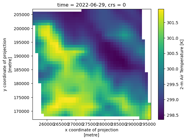
Dimensions:   (time: 7306, x: 41, y: 40)
Coordinates:
  * time      (time) datetime64[ns] 2022-06-29 ... 2023-04-29T10:00:00
  * x         (x) float64 2.555e+05 2.565e+05 2.575e+05 ... 2.945e+05 2.955e+05
  * y         (y) float64 1.675e+05 1.685e+05 1.695e+05 ... 2.055e+05 2.065e+05
    crs       int64 0
Data variables:
    LWDOWN    (time, y, x) float64 dask.array<chunksize=(168, 40, 33), meta=np.ndarray>
    PSFC      (time, y, x) float64 dask.array<chunksize=(168, 40, 33), meta=np.ndarray>
    Q2D       (time, y, x) float64 dask.array<chunksize=(168, 40, 33), meta=np.ndarray>
    RAINRATE  (time, y, x) float32 dask.array<chunksize=(168, 40, 33), meta=np.ndarray>
    SWDOWN    (time, y, x) float64 dask.array<chunksize=(168, 40, 33), meta=np.ndarray>
    T2D       (time, y, x) float64 dask.array<chunksize=(168, 40, 33), meta=np.ndarray>
    U2D       (time, y, x) float64 dask.array<chunksize=(168, 40, 33), meta=np.ndarray>
    V2D       (time, y, x) float64 dask.array<chunksize=(168, 40, 33), meta=np.ndarray>
Attributes:
    NWM_version_number:         v2.2
    model_configuration:        short_range
    model_initialization_time:  2023-04-27_11:00:00
    model_output_type:          forcing
    model_output_valid_time:    2023-04-27_12:00:00
    model_total_valid_times:    18
    pangeo-forge:inputs_hash:   59784c1feed1b881dc936b070ac5a83cbc680599cb9b6...
    pangeo-forge:recipe_hash:   25e9980cd34a6a0871883fc7375f224d34f403c944f95...
    pangeo-forge:version:       0.9.4

xarray.Dataset

• Dimensions:
  • time: 7306
  • x: 41
  • y: 40
• Coordinates: (4)
  • time
    (time)
    datetime64[ns]
    2022-06-29 ... 2023-04-29T10:00:00

    array(['2022-06-29T00:00:00.000000000', '2022-06-29T01:00:00.000000000',
           '2022-06-29T02:00:00.000000000', ..., '2023-04-29T08:00:00.000000000',
           '2023-04-29T09:00:00.000000000', '2023-04-29T10:00:00.000000000'],
          dtype='datetime64[ns]')

  • x
    (x)
    float64
    2.555e+05 2.565e+05 ... 2.955e+05

    _CoordinateAxisType :

    GeoX

    long_name :

    x coordinate of projection

    resolution :

    1000.0

    standard_name :

    projection_x_coordinate

    units :

    metre

    axis :

    X

    array([255500.828125, 256500.828125, 257500.828125, 258500.828125,
           259500.828125, 260500.828125, 261500.828125, 262500.8125  ,
           263500.8125  , 264500.8125  , 265500.8125  , 266500.8125  ,
           267500.8125  , 268500.8125  , 269500.8125  , 270500.8125  ,
           271500.8125  , 272500.8125  , 273500.8125  , 274500.8125  ,
           275500.8125  , 276500.8125  , 277500.8125  , 278500.8125  ,
           279500.8125  , 280500.8125  , 281500.8125  , 282500.8125  ,
           283500.8125  , 284500.8125  , 285500.8125  , 286500.8125  ,
           287500.8125  , 288500.8125  , 289500.8125  , 290500.8125  ,
           291500.8125  , 292500.8125  , 293500.8125  , 294500.8125  ,
           295500.8125  ])

  • y
    (y)
    float64
    1.675e+05 1.685e+05 ... 2.065e+05

    _CoordinateAxisType :

    GeoY

    long_name :

    y coordinate of projection

    resolution :

    1000.0

    standard_name :

    projection_y_coordinate

    units :

    metre

    axis :

    Y

    array([167499.65625, 168499.65625, 169499.65625, 170499.65625, 171499.65625,
           172499.65625, 173499.65625, 174499.65625, 175499.65625, 176499.65625,
           177499.65625, 178499.65625, 179499.65625, 180499.65625, 181499.65625,
           182499.65625, 183499.65625, 184499.65625, 185499.65625, 186499.65625,
           187499.65625, 188499.65625, 189499.65625, 190499.65625, 191499.65625,
           192499.65625, 193499.65625, 194499.65625, 195499.65625, 196499.65625,
           197499.65625, 198499.65625, 199499.65625, 200499.65625, 201499.65625,
           202499.65625, 203499.65625, 204499.65625, 205499.65625, 206499.65625])

  • crs
    ()
    int64
    0

    crs_wkt :

    PROJCS["Lambert_Conformal_Conic",GEOGCS["Unknown datum based upon the Authalic Sphere",DATUM["Not_specified_based_on_Authalic_Sphere",SPHEROID["Sphere",6370000,0],AUTHORITY["EPSG","6035"]],PRIMEM["Greenwich",0],UNIT["Degree",0.0174532925199433]],PROJECTION["Lambert_Conformal_Conic_2SP"],PARAMETER["false_easting",0],PARAMETER["false_northing",0],PARAMETER["central_meridian",-97],PARAMETER["standard_parallel_1",30],PARAMETER["standard_parallel_2",60],PARAMETER["latitude_of_origin",40],UNIT["metre",1,AUTHORITY["EPSG","9001"]],AXIS["Easting",EAST],AXIS["Northing",NORTH]]

    semi_major_axis :

    6370000.0

    semi_minor_axis :

    6370000.0

    inverse_flattening :

    0.0

    reference_ellipsoid_name :

    Sphere

    longitude_of_prime_meridian :

    0.0

    prime_meridian_name :

    Greenwich

    geographic_crs_name :

    Unknown datum based upon the Authalic Sphere

    horizontal_datum_name :

    Not specified (based on Authalic Sphere)

    projected_crs_name :

    Lambert_Conformal_Conic

    grid_mapping_name :

    lambert_conformal_conic

    standard_parallel :

    (30.0, 60.0)

    latitude_of_projection_origin :

    40.0

    longitude_of_central_meridian :

    -97.0

    false_easting :

    0.0

    false_northing :

    0.0

    spatial_ref :

    PROJCS["Lambert_Conformal_Conic",GEOGCS["Unknown datum based upon the Authalic Sphere",DATUM["Not_specified_based_on_Authalic_Sphere",SPHEROID["Sphere",6370000,0],AUTHORITY["EPSG","6035"]],PRIMEM["Greenwich",0],UNIT["Degree",0.0174532925199433]],PROJECTION["Lambert_Conformal_Conic_2SP"],PARAMETER["false_easting",0],PARAMETER["false_northing",0],PARAMETER["central_meridian",-97],PARAMETER["standard_parallel_1",30],PARAMETER["standard_parallel_2",60],PARAMETER["latitude_of_origin",40],UNIT["metre",1,AUTHORITY["EPSG","9001"]],AXIS["Easting",EAST],AXIS["Northing",NORTH]]

    GeoTransform :

    255000.8283203125 999.999609375 0.0 166999.65625 0.0 1000.0

    array(0)

• Data variables: (8)
  • LWDOWN
    (time, y, x)
    float64
    dask.array<chunksize=(168, 40, 33), meta=np.ndarray>

    cell_methods :

    time: point

    esri_pe_string :

    PROJCS["Lambert_Conformal_Conic",GEOGCS["GCS_Sphere",DATUM["D_Sphere",SPHEROID["Sphere",6370000.0,0.0]],PRIMEM["Greenwich",0.0],UNIT["Degree",0.0174532925199433]],PROJECTION["Lambert_Conformal_Conic_2SP"],PARAMETER["false_easting",0.0],PARAMETER["false_northing",0.0],PARAMETER["central_meridian",-97.0],PARAMETER["standard_parallel_1",30.0],PARAMETER["standard_parallel_2",60.0],PARAMETER["latitude_of_origin",40.0],UNIT["Meter",1.0]];-35691800 -29075200 10000;-100000 10000;-100000 10000;0.001;0.001;0.001;IsHighPrecision

    grid_mapping :

    crs

    long_name :

    Surface downward long-wave radiation flux

    proj4 :

    +proj=lcc +units=m +a=6370000.0 +b=6370000.0 +lat_1=30.0 +lat_2=60.0 +lat_0=40.0 +lon_0=-97.0 +x_0=0 +y_0=0 +k_0=1.0 +nadgrids=@null +wktext +no_defs

    remap :

    remapped via ESMF regrid_with_weights: Bilinear

    standard_name :

    surface_downward_longwave_flux

    units :

    W m-2

    Array Chunk Bytes 91.41 MiB 1.69 MiB Shape (7306, 40, 41) (168, 40, 33) Dask graph 88 chunks in 6 graph layers Data type float64 numpy.ndarray

  • PSFC
    (time, y, x)
    float64
    dask.array<chunksize=(168, 40, 33), meta=np.ndarray>

    cell_methods :

    time: point

    esri_pe_string :

    PROJCS["Lambert_Conformal_Conic",GEOGCS["GCS_Sphere",DATUM["D_Sphere",SPHEROID["Sphere",6370000.0,0.0]],PRIMEM["Greenwich",0.0],UNIT["Degree",0.0174532925199433]],PROJECTION["Lambert_Conformal_Conic_2SP"],PARAMETER["false_easting",0.0],PARAMETER["false_northing",0.0],PARAMETER["central_meridian",-97.0],PARAMETER["standard_parallel_1",30.0],PARAMETER["standard_parallel_2",60.0],PARAMETER["latitude_of_origin",40.0],UNIT["Meter",1.0]];-35691800 -29075200 10000;-100000 10000;-100000 10000;0.001;0.001;0.001;IsHighPrecision

    grid_mapping :

    crs

    long_name :

    Surface Pressure

    proj4 :

    +proj=lcc +units=m +a=6370000.0 +b=6370000.0 +lat_1=30.0 +lat_2=60.0 +lat_0=40.0 +lon_0=-97.0 +x_0=0 +y_0=0 +k_0=1.0 +nadgrids=@null +wktext +no_defs

    remap :

    remapped via ESMF regrid_with_weights: Bilinear

    standard_name :

    air_pressure

    units :

    Pa

    Array Chunk Bytes 91.41 MiB 1.69 MiB Shape (7306, 40, 41) (168, 40, 33) Dask graph 88 chunks in 6 graph layers Data type float64 numpy.ndarray

  • Q2D
    (time, y, x)
    float64
    dask.array<chunksize=(168, 40, 33), meta=np.ndarray>

    cell_methods :

    time: point

    esri_pe_string :

    PROJCS["Lambert_Conformal_Conic",GEOGCS["GCS_Sphere",DATUM["D_Sphere",SPHEROID["Sphere",6370000.0,0.0]],PRIMEM["Greenwich",0.0],UNIT["Degree",0.0174532925199433]],PROJECTION["Lambert_Conformal_Conic_2SP"],PARAMETER["false_easting",0.0],PARAMETER["false_northing",0.0],PARAMETER["central_meridian",-97.0],PARAMETER["standard_parallel_1",30.0],PARAMETER["standard_parallel_2",60.0],PARAMETER["latitude_of_origin",40.0],UNIT["Meter",1.0]];-35691800 -29075200 10000;-100000 10000;-100000 10000;0.001;0.001;0.001;IsHighPrecision

    grid_mapping :

    crs

    long_name :

    2-m Specific Humidity

    proj4 :

    +proj=lcc +units=m +a=6370000.0 +b=6370000.0 +lat_1=30.0 +lat_2=60.0 +lat_0=40.0 +lon_0=-97.0 +x_0=0 +y_0=0 +k_0=1.0 +nadgrids=@null +wktext +no_defs

    remap :

    remapped via ESMF regrid_with_weights: Bilinear

    standard_name :

    surface_specific_humidity

    units :

    kg kg-1

    Array Chunk Bytes 91.41 MiB 1.69 MiB Shape (7306, 40, 41) (168, 40, 33) Dask graph 88 chunks in 6 graph layers Data type float64 numpy.ndarray

  • RAINRATE
    (time, y, x)
    float32
    dask.array<chunksize=(168, 40, 33), meta=np.ndarray>

    cell_methods :

    time: mean

    esri_pe_string :

    PROJCS["Lambert_Conformal_Conic",GEOGCS["GCS_Sphere",DATUM["D_Sphere",SPHEROID["Sphere",6370000.0,0.0]],PRIMEM["Greenwich",0.0],UNIT["Degree",0.0174532925199433]],PROJECTION["Lambert_Conformal_Conic_2SP"],PARAMETER["false_easting",0.0],PARAMETER["false_northing",0.0],PARAMETER["central_meridian",-97.0],PARAMETER["standard_parallel_1",30.0],PARAMETER["standard_parallel_2",60.0],PARAMETER["latitude_of_origin",40.0],UNIT["Meter",1.0]];-35691800 -29075200 10000;-100000 10000;-100000 10000;0.001;0.001;0.001;IsHighPrecision

    grid_mapping :

    crs

    long_name :

    Surface Precipitation Rate

    proj4 :

    +proj=lcc +units=m +a=6370000.0 +b=6370000.0 +lat_1=30.0 +lat_2=60.0 +lat_0=40.0 +lon_0=-97.0 +x_0=0 +y_0=0 +k_0=1.0 +nadgrids=@null +wktext +no_defs

    remap :

    remapped via ESMF regrid_with_weights: Bilinear

    standard_name :

    precipitation_flux

    units :

    mm s^-1

    Array Chunk Bytes 45.71 MiB 866.25 kiB Shape (7306, 40, 41) (168, 40, 33) Dask graph 88 chunks in 6 graph layers Data type float32 numpy.ndarray

  • SWDOWN
    (time, y, x)
    float64
    dask.array<chunksize=(168, 40, 33), meta=np.ndarray>

    cell_methods :

    time point

    esri_pe_string :

    PROJCS["Lambert_Conformal_Conic",GEOGCS["GCS_Sphere",DATUM["D_Sphere",SPHEROID["Sphere",6370000.0,0.0]],PRIMEM["Greenwich",0.0],UNIT["Degree",0.0174532925199433]],PROJECTION["Lambert_Conformal_Conic_2SP"],PARAMETER["false_easting",0.0],PARAMETER["false_northing",0.0],PARAMETER["central_meridian",-97.0],PARAMETER["standard_parallel_1",30.0],PARAMETER["standard_parallel_2",60.0],PARAMETER["latitude_of_origin",40.0],UNIT["Meter",1.0]];-35691800 -29075200 10000;-100000 10000;-100000 10000;0.001;0.001;0.001;IsHighPrecision

    grid_mapping :

    crs

    long_name :

    Surface downward short-wave radiation flux

    proj4 :

    +proj=lcc +units=m +a=6370000.0 +b=6370000.0 +lat_1=30.0 +lat_2=60.0 +lat_0=40.0 +lon_0=-97.0 +x_0=0 +y_0=0 +k_0=1.0 +nadgrids=@null +wktext +no_defs

    remap :

    remapped via ESMF regrid_with_weights: Bilinear

    standard_name :

    surface_downward_shortwave_flux

    units :

    W m-2

    Array Chunk Bytes 91.41 MiB 1.69 MiB Shape (7306, 40, 41) (168, 40, 33) Dask graph 88 chunks in 6 graph layers Data type float64 numpy.ndarray

  • T2D
    (time, y, x)
    float64
    dask.array<chunksize=(168, 40, 33), meta=np.ndarray>

    cell_methods :

    time: point

    esri_pe_string :

    PROJCS["Lambert_Conformal_Conic",GEOGCS["GCS_Sphere",DATUM["D_Sphere",SPHEROID["Sphere",6370000.0,0.0]],PRIMEM["Greenwich",0.0],UNIT["Degree",0.0174532925199433]],PROJECTION["Lambert_Conformal_Conic_2SP"],PARAMETER["false_easting",0.0],PARAMETER["false_northing",0.0],PARAMETER["central_meridian",-97.0],PARAMETER["standard_parallel_1",30.0],PARAMETER["standard_parallel_2",60.0],PARAMETER["latitude_of_origin",40.0],UNIT["Meter",1.0]];-35691800 -29075200 10000;-100000 10000;-100000 10000;0.001;0.001;0.001;IsHighPrecision

    grid_mapping :

    crs

    long_name :

    2-m Air Temperature

    proj4 :

    +proj=lcc +units=m +a=6370000.0 +b=6370000.0 +lat_1=30.0 +lat_2=60.0 +lat_0=40.0 +lon_0=-97.0 +x_0=0 +y_0=0 +k_0=1.0 +nadgrids=@null +wktext +no_defs

    remap :

    remapped via ESMF regrid_with_weights: Bilinear

    standard_name :

    air_temperature

    units :

    K

    Array Chunk Bytes 91.41 MiB 1.69 MiB Shape (7306, 40, 41) (168, 40, 33) Dask graph 88 chunks in 6 graph layers Data type float64 numpy.ndarray

  • U2D
    (time, y, x)
    float64
    dask.array<chunksize=(168, 40, 33), meta=np.ndarray>

    cell_methods :

    time: point

    esri_pe_string :

    PROJCS["Lambert_Conformal_Conic",GEOGCS["GCS_Sphere",DATUM["D_Sphere",SPHEROID["Sphere",6370000.0,0.0]],PRIMEM["Greenwich",0.0],UNIT["Degree",0.0174532925199433]],PROJECTION["Lambert_Conformal_Conic_2SP"],PARAMETER["false_easting",0.0],PARAMETER["false_northing",0.0],PARAMETER["central_meridian",-97.0],PARAMETER["standard_parallel_1",30.0],PARAMETER["standard_parallel_2",60.0],PARAMETER["latitude_of_origin",40.0],UNIT["Meter",1.0]];-35691800 -29075200 10000;-100000 10000;-100000 10000;0.001;0.001;0.001;IsHighPrecision

    grid_mapping :

    crs

    long_name :

    10-m U-component of wind

    proj4 :

    +proj=lcc +units=m +a=6370000.0 +b=6370000.0 +lat_1=30.0 +lat_2=60.0 +lat_0=40.0 +lon_0=-97.0 +x_0=0 +y_0=0 +k_0=1.0 +nadgrids=@null +wktext +no_defs

    remap :

    remapped via ESMF regrid_with_weights: Bilinear

    standard_name :

    x_wind

    units :

    m s-1

    Array Chunk Bytes 91.41 MiB 1.69 MiB Shape (7306, 40, 41) (168, 40, 33) Dask graph 88 chunks in 6 graph layers Data type float64 numpy.ndarray

  • V2D
    (time, y, x)
    float64
    dask.array<chunksize=(168, 40, 33), meta=np.ndarray>

    cell_methods :

    time: point

    esri_pe_string :

    PROJCS["Lambert_Conformal_Conic",GEOGCS["GCS_Sphere",DATUM["D_Sphere",SPHEROID["Sphere",6370000.0,0.0]],PRIMEM["Greenwich",0.0],UNIT["Degree",0.0174532925199433]],PROJECTION["Lambert_Conformal_Conic_2SP"],PARAMETER["false_easting",0.0],PARAMETER["false_northing",0.0],PARAMETER["central_meridian",-97.0],PARAMETER["standard_parallel_1",30.0],PARAMETER["standard_parallel_2",60.0],PARAMETER["latitude_of_origin",40.0],UNIT["Meter",1.0]];-35691800 -29075200 10000;-100000 10000;-100000 10000;0.001;0.001;0.001;IsHighPrecision

    grid_mapping :

    crs

    long_name :

    10-m V-component of wind

    proj4 :

    +proj=lcc +units=m +a=6370000.0 +b=6370000.0 +lat_1=30.0 +lat_2=60.0 +lat_0=40.0 +lon_0=-97.0 +x_0=0 +y_0=0 +k_0=1.0 +nadgrids=@null +wktext +no_defs

    remap :

    remapped via ESMF regrid_with_weights: Bilinear

    standard_name :

    y_wind

    units :

    m s-1

    Array Chunk Bytes 91.41 MiB 1.69 MiB Shape (7306, 40, 41) (168, 40, 33) Dask graph 88 chunks in 6 graph layers Data type float64 numpy.ndarray

• Indexes: (3)
  • time
    PandasIndex

    PandasIndex(DatetimeIndex(['2022-06-29 00:00:00', '2022-06-29 01:00:00',
                   '2022-06-29 02:00:00', '2022-06-29 03:00:00',
                   '2022-06-29 04:00:00', '2022-06-29 05:00:00',
                   '2022-06-29 06:00:00', '2022-06-29 07:00:00',
                   '2022-06-29 08:00:00', '2022-06-29 09:00:00',
                   ...
                   '2023-04-29 01:00:00', '2023-04-29 02:00:00',
                   '2023-04-29 03:00:00', '2023-04-29 04:00:00',
                   '2023-04-29 05:00:00', '2023-04-29 06:00:00',
                   '2023-04-29 07:00:00', '2023-04-29 08:00:00',
                   '2023-04-29 09:00:00', '2023-04-29 10:00:00'],
                  dtype='datetime64[ns]', name='time', length=7306, freq=None))

  • x
    PandasIndex

    PandasIndex(Index([255500.828125, 256500.828125, 257500.828125, 258500.828125,
           259500.828125, 260500.828125, 261500.828125,   262500.8125,
             263500.8125,   264500.8125,   265500.8125,   266500.8125,
             267500.8125,   268500.8125,   269500.8125,   270500.8125,
             271500.8125,   272500.8125,   273500.8125,   274500.8125,
             275500.8125,   276500.8125,   277500.8125,   278500.8125,
             279500.8125,   280500.8125,   281500.8125,   282500.8125,
             283500.8125,   284500.8125,   285500.8125,   286500.8125,
             287500.8125,   288500.8125,   289500.8125,   290500.8125,
             291500.8125,   292500.8125,   293500.8125,   294500.8125,
             295500.8125],
          dtype='float64', name='x'))

  • y
    PandasIndex

    PandasIndex(Index([167499.65625, 168499.65625, 169499.65625, 170499.65625, 171499.65625,
           172499.65625, 173499.65625, 174499.65625, 175499.65625, 176499.65625,
           177499.65625, 178499.65625, 179499.65625, 180499.65625, 181499.65625,
           182499.65625, 183499.65625, 184499.65625, 185499.65625, 186499.65625,
           187499.65625, 188499.65625, 189499.65625, 190499.65625, 191499.65625,
           192499.65625, 193499.65625, 194499.65625, 195499.65625, 196499.65625,
           197499.65625, 198499.65625, 199499.65625, 200499.65625, 201499.65625,
           202499.65625, 203499.65625, 204499.65625, 205499.65625, 206499.65625],
          dtype='float64', name='y'))

• Attributes: (9)

  NWM_version_number :

  v2.2

  model_configuration :

  short_range

  model_initialization_time :

  2023-04-27_11:00:00

  model_output_type :

  forcing

  model_output_valid_time :

  2023-04-27_12:00:00

  model_total_valid_times :

  18

  pangeo-forge:inputs_hash :

  59784c1feed1b881dc936b070ac5a83cbc680599cb9b65b9f61dae68777a174f

  pangeo-forge:recipe_hash :

  25e9980cd34a6a0871883fc7375f224d34f403c944f9578ac5b8caea697170c8

  pangeo-forge:version :

  0.9.4

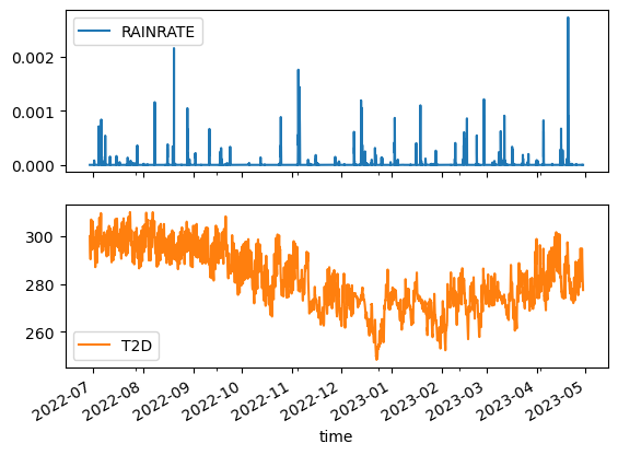
Accessing a single timestamp of data from this subset is fast:

ts.T2D.isel(time=0).plot();

Accessing data through time is also relatively fast (compared to using the dataset that’s chunked in time).

from distributed import Client

client = Client()
client

Client

Client-632558ef-f4bf-11ed-83c7-32bb6486e0f8

Connection method: Cluster object	Cluster type: distributed.LocalCluster
Dashboard: /user/taugspurger/proxy/8787/status

Launch dashboard in JupyterLab

Cluster Info

LocalCluster

67d77040

Dashboard: /user/taugspurger/proxy/8787/status	Workers: 4
Total threads: 8	Total memory: 7.50 GiB
Status: running	Using processes: True

Scheduler Info

Scheduler

Scheduler-f6320a91-76fc-4263-add6-d560952fadca

Comm: tcp://127.0.0.1:37413	Workers: 4
Dashboard: /user/taugspurger/proxy/8787/status	Total threads: 8
Started: Just now	Total memory: 7.50 GiB

Workers

Worker: 0

Comm: tcp://127.0.0.1:46111	Total threads: 2
Dashboard: /user/taugspurger/proxy/34917/status	Memory: 1.88 GiB
Nanny: tcp://127.0.0.1:33065
Local directory: /tmp/dask-worker-space/worker-vumqckxz

Worker: 1

Comm: tcp://127.0.0.1:45429	Total threads: 2
Dashboard: /user/taugspurger/proxy/44995/status	Memory: 1.88 GiB
Nanny: tcp://127.0.0.1:34179
Local directory: /tmp/dask-worker-space/worker-xbn6qzu4

Worker: 2

Comm: tcp://127.0.0.1:38817	Total threads: 2
Dashboard: /user/taugspurger/proxy/41733/status	Memory: 1.88 GiB
Nanny: tcp://127.0.0.1:39513
Local directory: /tmp/dask-worker-space/worker-_k5g9cyp

Worker: 3

Comm: tcp://127.0.0.1:35347	Total threads: 2
Dashboard: /user/taugspurger/proxy/40943/status	Memory: 1.88 GiB
Nanny: tcp://127.0.0.1:45679
Local directory: /tmp/dask-worker-space/worker-ob5iaaus

t = ts[["RAINRATE", "T2D"]].mean(dim=("y", "x")).compute()

t.to_dataframe()[["RAINRATE", "T2D"]].plot(subplots=True);

client.close()

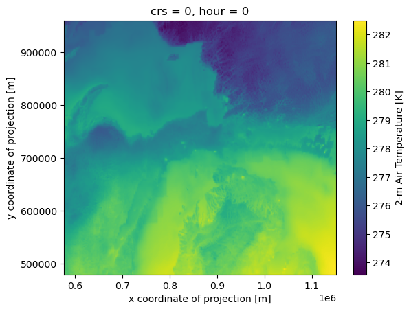
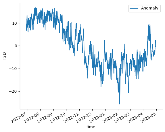
Now let’s do a fun computation. We’ll calculate an average temperature at each hour, and look at the difference (anomaly?) from it over the course of our timeseries.

This will be a large computation, so let’s parallelize it on a cluster.

from dask_gateway import GatewayCluster

cluster = GatewayCluster()
cluster.scale(16)
client = cluster.get_client()
client

Client

Client-7e49bf19-f4bf-11ed-83c7-32bb6486e0f8

Connection method: Cluster object	Cluster type: dask_gateway.GatewayCluster
Dashboard: /services/dask-gateway/clusters/default.c0d5d67063384fe2acdb71d0e6615657/status

Launch dashboard in JupyterLab

Cluster Info

GatewayCluster

• Name: default.c0d5d67063384fe2acdb71d0e6615657
• Dashboard: /services/dask-gateway/clusters/default.c0d5d67063384fe2acdb71d0e6615657/status

subset = ds["T2D"].isel(y=slice(2400, 2880), x=slice(2880, 3456))
subset

<xarray.DataArray 'T2D' (time: 7306, y: 480, x: 576)>
dask.array<getitem, shape=(7306, 480, 576), dtype=float64, chunksize=(168, 240, 288), chunktype=numpy.ndarray>
Coordinates:
    crs      int64 0
  * time     (time) datetime64[ns] 2022-06-29 ... 2023-04-29T10:00:00
  * x        (x) float64 5.765e+05 5.775e+05 5.785e+05 ... 1.151e+06 1.152e+06
  * y        (y) float64 4.805e+05 4.815e+05 4.825e+05 ... 9.585e+05 9.595e+05
Attributes:
    cell_methods:    time: point
    esri_pe_string:  PROJCS["Lambert_Conformal_Conic",GEOGCS["GCS_Sphere",DAT...
    grid_mapping:    crs
    long_name:       2-m Air Temperature
    proj4:           +proj=lcc +units=m +a=6370000.0 +b=6370000.0 +lat_1=30.0...
    remap:           remapped via ESMF regrid_with_weights: Bilinear
    standard_name:   air_temperature
    units:           K

xarray.DataArray

'T2D'

• time: 7306
• y: 480
• x: 576

• dask.array<chunksize=(168, 240, 288), meta=np.ndarray>

  Array Chunk Bytes 15.05 GiB 88.59 MiB Shape (7306, 480, 576) (168, 240, 288) Dask graph 176 chunks in 3 graph layers Data type float64 numpy.ndarray

• Coordinates: (4)
  • crs
    ()
    int64
    0

    crs_wkt :

    PROJCS["Lambert_Conformal_Conic",GEOGCS["Unknown datum based upon the Authalic Sphere",DATUM["Not_specified_based_on_Authalic_Sphere",SPHEROID["Sphere",6370000,0],AUTHORITY["EPSG","6035"]],PRIMEM["Greenwich",0],UNIT["Degree",0.0174532925199433]],PROJECTION["Lambert_Conformal_Conic_2SP"],PARAMETER["false_easting",0],PARAMETER["false_northing",0],PARAMETER["central_meridian",-97],PARAMETER["standard_parallel_1",30],PARAMETER["standard_parallel_2",60],PARAMETER["latitude_of_origin",40],UNIT["metre",1,AUTHORITY["EPSG","9001"]],AXIS["Easting",EAST],AXIS["Northing",NORTH]]

    semi_major_axis :

    6370000.0

    semi_minor_axis :

    6370000.0

    inverse_flattening :

    0.0

    reference_ellipsoid_name :

    Sphere

    longitude_of_prime_meridian :

    0.0

    prime_meridian_name :

    Greenwich

    geographic_crs_name :

    Unknown datum based upon the Authalic Sphere

    horizontal_datum_name :

    Not specified (based on Authalic Sphere)

    projected_crs_name :

    Lambert_Conformal_Conic

    grid_mapping_name :

    lambert_conformal_conic

    standard_parallel :

    (30.0, 60.0)

    latitude_of_projection_origin :

    40.0

    longitude_of_central_meridian :

    -97.0

    false_easting :

    0.0

    false_northing :

    0.0

    spatial_ref :

    PROJCS["Lambert_Conformal_Conic",GEOGCS["Unknown datum based upon the Authalic Sphere",DATUM["Not_specified_based_on_Authalic_Sphere",SPHEROID["Sphere",6370000,0],AUTHORITY["EPSG","6035"]],PRIMEM["Greenwich",0],UNIT["Degree",0.0174532925199433]],PROJECTION["Lambert_Conformal_Conic_2SP"],PARAMETER["false_easting",0],PARAMETER["false_northing",0],PARAMETER["central_meridian",-97],PARAMETER["standard_parallel_1",30],PARAMETER["standard_parallel_2",60],PARAMETER["latitude_of_origin",40],UNIT["metre",1,AUTHORITY["EPSG","9001"]],AXIS["Easting",EAST],AXIS["Northing",NORTH]]

    array(0)

  • time
    (time)
    datetime64[ns]
    2022-06-29 ... 2023-04-29T10:00:00

    array(['2022-06-29T00:00:00.000000000', '2022-06-29T01:00:00.000000000',
           '2022-06-29T02:00:00.000000000', ..., '2023-04-29T08:00:00.000000000',
           '2023-04-29T09:00:00.000000000', '2023-04-29T10:00:00.000000000'],
          dtype='datetime64[ns]')

  • x
    (x)
    float64
    5.765e+05 5.775e+05 ... 1.152e+06

    _CoordinateAxisType :

    GeoX

    long_name :

    x coordinate of projection

    resolution :

    1000.0

    standard_name :

    projection_x_coordinate

    units :

    m

    array([ 576500.8125,  577500.8125,  578500.8125, ..., 1149500.875 ,
           1150500.875 , 1151500.875 ])

  • y
    (y)
    float64
    4.805e+05 4.815e+05 ... 9.595e+05

    _CoordinateAxisType :

    GeoY

    long_name :

    y coordinate of projection

    resolution :

    1000.0

    standard_name :

    projection_y_coordinate

    units :

    m

    array([480499.65625, 481499.65625, 482499.65625, ..., 957499.6875 ,
           958499.6875 , 959499.6875 ])

• Indexes: (3)
  • time
    PandasIndex

    PandasIndex(DatetimeIndex(['2022-06-29 00:00:00', '2022-06-29 01:00:00',
                   '2022-06-29 02:00:00', '2022-06-29 03:00:00',
                   '2022-06-29 04:00:00', '2022-06-29 05:00:00',
                   '2022-06-29 06:00:00', '2022-06-29 07:00:00',
                   '2022-06-29 08:00:00', '2022-06-29 09:00:00',
                   ...
                   '2023-04-29 01:00:00', '2023-04-29 02:00:00',
                   '2023-04-29 03:00:00', '2023-04-29 04:00:00',
                   '2023-04-29 05:00:00', '2023-04-29 06:00:00',
                   '2023-04-29 07:00:00', '2023-04-29 08:00:00',
                   '2023-04-29 09:00:00', '2023-04-29 10:00:00'],
                  dtype='datetime64[ns]', name='time', length=7306, freq=None))

  • x
    PandasIndex

    PandasIndex(Index([576500.8125, 577500.8125, 578500.8125, 579500.8125, 580500.8125,
           581500.8125, 582500.8125, 583500.8125, 584500.8125, 585500.8125,
           ...
           1142500.875, 1143500.875, 1144500.875, 1145500.875, 1146500.875,
           1147500.875, 1148500.875, 1149500.875, 1150500.875, 1151500.875],
          dtype='float64', name='x', length=576))

  • y
    PandasIndex

    PandasIndex(Index([480499.65625, 481499.65625, 482499.65625, 483499.65625, 484499.65625,
           485499.65625, 486499.65625, 487499.65625, 488499.65625, 489499.65625,
           ...
            950499.6875,  951499.6875,  952499.6875,  953499.6875,  954499.6875,
            955499.6875,  956499.6875,  957499.6875,  958499.6875,  959499.6875],
          dtype='float64', name='y', length=480))

• Attributes: (8)

  cell_methods :

  time: point

  esri_pe_string :

  PROJCS["Lambert_Conformal_Conic",GEOGCS["GCS_Sphere",DATUM["D_Sphere",SPHEROID["Sphere",6370000.0,0.0]],PRIMEM["Greenwich",0.0],UNIT["Degree",0.0174532925199433]],PROJECTION["Lambert_Conformal_Conic_2SP"],PARAMETER["false_easting",0.0],PARAMETER["false_northing",0.0],PARAMETER["central_meridian",-97.0],PARAMETER["standard_parallel_1",30.0],PARAMETER["standard_parallel_2",60.0],PARAMETER["latitude_of_origin",40.0],UNIT["Meter",1.0]];-35691800 -29075200 10000;-100000 10000;-100000 10000;0.001;0.001;0.001;IsHighPrecision

  grid_mapping :

  crs

  long_name :

  2-m Air Temperature

  proj4 :

  +proj=lcc +units=m +a=6370000.0 +b=6370000.0 +lat_1=30.0 +lat_2=60.0 +lat_0=40.0 +lon_0=-97.0 +x_0=0 +y_0=0 +k_0=1.0 +nadgrids=@null +wktext +no_defs

  remap :

  remapped via ESMF regrid_with_weights: Bilinear

  standard_name :

  air_temperature

  units :

  K

hourly = subset.groupby("time.hour").mean(dim="time")
hourly

<xarray.DataArray 'T2D' (hour: 24, y: 480, x: 576)>
dask.array<transpose, shape=(24, 480, 576), dtype=float64, chunksize=(24, 240, 288), chunktype=numpy.ndarray>
Coordinates:
    crs      int64 0
  * x        (x) float64 5.765e+05 5.775e+05 5.785e+05 ... 1.151e+06 1.152e+06
  * y        (y) float64 4.805e+05 4.815e+05 4.825e+05 ... 9.585e+05 9.595e+05
  * hour     (hour) int64 0 1 2 3 4 5 6 7 8 9 ... 14 15 16 17 18 19 20 21 22 23
Attributes:
    cell_methods:    time: point
    esri_pe_string:  PROJCS["Lambert_Conformal_Conic",GEOGCS["GCS_Sphere",DAT...
    grid_mapping:    crs
    long_name:       2-m Air Temperature
    proj4:           +proj=lcc +units=m +a=6370000.0 +b=6370000.0 +lat_1=30.0...
    remap:           remapped via ESMF regrid_with_weights: Bilinear
    standard_name:   air_temperature
    units:           K

xarray.DataArray

'T2D'

• hour: 24
• y: 480
• x: 576

• dask.array<chunksize=(24, 240, 288), meta=np.ndarray>

  Array Chunk Bytes 50.62 MiB 12.66 MiB Shape (24, 480, 576) (24, 240, 288) Dask graph 4 chunks in 13 graph layers Data type float64 numpy.ndarray

• Coordinates: (4)
  • crs
    ()
    int64
    0

    crs_wkt :

    PROJCS["Lambert_Conformal_Conic",GEOGCS["Unknown datum based upon the Authalic Sphere",DATUM["Not_specified_based_on_Authalic_Sphere",SPHEROID["Sphere",6370000,0],AUTHORITY["EPSG","6035"]],PRIMEM["Greenwich",0],UNIT["Degree",0.0174532925199433]],PROJECTION["Lambert_Conformal_Conic_2SP"],PARAMETER["false_easting",0],PARAMETER["false_northing",0],PARAMETER["central_meridian",-97],PARAMETER["standard_parallel_1",30],PARAMETER["standard_parallel_2",60],PARAMETER["latitude_of_origin",40],UNIT["metre",1,AUTHORITY["EPSG","9001"]],AXIS["Easting",EAST],AXIS["Northing",NORTH]]

    semi_major_axis :

    6370000.0

    semi_minor_axis :

    6370000.0

    inverse_flattening :

    0.0

    reference_ellipsoid_name :

    Sphere

    longitude_of_prime_meridian :

    0.0

    prime_meridian_name :

    Greenwich

    geographic_crs_name :

    Unknown datum based upon the Authalic Sphere

    horizontal_datum_name :

    Not specified (based on Authalic Sphere)

    projected_crs_name :

    Lambert_Conformal_Conic

    grid_mapping_name :

    lambert_conformal_conic

    standard_parallel :

    (30.0, 60.0)

    latitude_of_projection_origin :

    40.0

    longitude_of_central_meridian :

    -97.0

    false_easting :

    0.0

    false_northing :

    0.0

    spatial_ref :

    PROJCS["Lambert_Conformal_Conic",GEOGCS["Unknown datum based upon the Authalic Sphere",DATUM["Not_specified_based_on_Authalic_Sphere",SPHEROID["Sphere",6370000,0],AUTHORITY["EPSG","6035"]],PRIMEM["Greenwich",0],UNIT["Degree",0.0174532925199433]],PROJECTION["Lambert_Conformal_Conic_2SP"],PARAMETER["false_easting",0],PARAMETER["false_northing",0],PARAMETER["central_meridian",-97],PARAMETER["standard_parallel_1",30],PARAMETER["standard_parallel_2",60],PARAMETER["latitude_of_origin",40],UNIT["metre",1,AUTHORITY["EPSG","9001"]],AXIS["Easting",EAST],AXIS["Northing",NORTH]]

    array(0)

  • x
    (x)
    float64
    5.765e+05 5.775e+05 ... 1.152e+06

    _CoordinateAxisType :

    GeoX

    long_name :

    x coordinate of projection

    resolution :

    1000.0

    standard_name :

    projection_x_coordinate

    units :

    m

    array([ 576500.8125,  577500.8125,  578500.8125, ..., 1149500.875 ,
           1150500.875 , 1151500.875 ])

  • y
    (y)
    float64
    4.805e+05 4.815e+05 ... 9.595e+05

    _CoordinateAxisType :

    GeoY

    long_name :

    y coordinate of projection

    resolution :

    1000.0

    standard_name :

    projection_y_coordinate

    units :

    m

    array([480499.65625, 481499.65625, 482499.65625, ..., 957499.6875 ,
           958499.6875 , 959499.6875 ])

  • hour
    (hour)
    int64
    0 1 2 3 4 5 6 ... 18 19 20 21 22 23

    array([ 0,  1,  2,  3,  4,  5,  6,  7,  8,  9, 10, 11, 12, 13, 14, 15, 16, 17,
           18, 19, 20, 21, 22, 23])

• Indexes: (3)
  • x
    PandasIndex

    PandasIndex(Index([576500.8125, 577500.8125, 578500.8125, 579500.8125, 580500.8125,
           581500.8125, 582500.8125, 583500.8125, 584500.8125, 585500.8125,
           ...
           1142500.875, 1143500.875, 1144500.875, 1145500.875, 1146500.875,
           1147500.875, 1148500.875, 1149500.875, 1150500.875, 1151500.875],
          dtype='float64', name='x', length=576))

  • y
    PandasIndex

    PandasIndex(Index([480499.65625, 481499.65625, 482499.65625, 483499.65625, 484499.65625,
           485499.65625, 486499.65625, 487499.65625, 488499.65625, 489499.65625,
           ...
            950499.6875,  951499.6875,  952499.6875,  953499.6875,  954499.6875,
            955499.6875,  956499.6875,  957499.6875,  958499.6875,  959499.6875],
          dtype='float64', name='y', length=480))

  • hour
    PandasIndex

    PandasIndex(Index([ 0,  1,  2,  3,  4,  5,  6,  7,  8,  9, 10, 11, 12, 13, 14, 15, 16, 17,
           18, 19, 20, 21, 22, 23],
          dtype='int64', name='hour'))

• Attributes: (8)

  cell_methods :

  time: point

  esri_pe_string :

  PROJCS["Lambert_Conformal_Conic",GEOGCS["GCS_Sphere",DATUM["D_Sphere",SPHEROID["Sphere",6370000.0,0.0]],PRIMEM["Greenwich",0.0],UNIT["Degree",0.0174532925199433]],PROJECTION["Lambert_Conformal_Conic_2SP"],PARAMETER["false_easting",0.0],PARAMETER["false_northing",0.0],PARAMETER["central_meridian",-97.0],PARAMETER["standard_parallel_1",30.0],PARAMETER["standard_parallel_2",60.0],PARAMETER["latitude_of_origin",40.0],UNIT["Meter",1.0]];-35691800 -29075200 10000;-100000 10000;-100000 10000;0.001;0.001;0.001;IsHighPrecision

  grid_mapping :

  crs

  long_name :

  2-m Air Temperature

  proj4 :

  +proj=lcc +units=m +a=6370000.0 +b=6370000.0 +lat_1=30.0 +lat_2=60.0 +lat_0=40.0 +lon_0=-97.0 +x_0=0 +y_0=0 +k_0=1.0 +nadgrids=@null +wktext +no_defs

  remap :

  remapped via ESMF regrid_with_weights: Bilinear

  standard_name :

  air_temperature

  units :

  K

We’ll use this result in a computation later on, so let’s persist it on the cluster.

hourly = hourly.persist()

And peek at the first timestamp.

hourly.isel(hour=0).plot();

Now we can calculate the anomaly.

import dask

with dask.config.set(**{"array.slicing.split_large_chunks": True}):
    anomaly = subset.groupby("time.hour") - hourly
anomaly

<xarray.DataArray 'T2D' (time: 7306, y: 480, x: 576)>
dask.array<sub, shape=(7306, 480, 576), dtype=float64, chunksize=(168, 240, 288), chunktype=numpy.ndarray>
Coordinates:
    crs      (time) int64 0 0 0 0 0 0 0 0 0 0 0 0 0 ... 0 0 0 0 0 0 0 0 0 0 0 0
  * time     (time) datetime64[ns] 2022-06-29 ... 2023-04-29T10:00:00
  * x        (x) float64 5.765e+05 5.775e+05 5.785e+05 ... 1.151e+06 1.152e+06
  * y        (y) float64 4.805e+05 4.815e+05 4.825e+05 ... 9.585e+05 9.595e+05
    hour     (time) int64 0 1 2 3 4 5 6 7 8 9 10 11 ... 0 1 2 3 4 5 6 7 8 9 10

xarray.DataArray

'T2D'

• time: 7306
• y: 480
• x: 576

• dask.array<chunksize=(168, 240, 288), meta=np.ndarray>

  Array Chunk Bytes 15.05 GiB 88.59 MiB Shape (7306, 480, 576) (168, 240, 288) Dask graph 296 chunks in 8 graph layers Data type float64 numpy.ndarray

• Coordinates: (5)
  • crs
    (time)
    int64
    0 0 0 0 0 0 0 0 ... 0 0 0 0 0 0 0 0

    crs_wkt :

    PROJCS["Lambert_Conformal_Conic",GEOGCS["Unknown datum based upon the Authalic Sphere",DATUM["Not_specified_based_on_Authalic_Sphere",SPHEROID["Sphere",6370000,0],AUTHORITY["EPSG","6035"]],PRIMEM["Greenwich",0],UNIT["Degree",0.0174532925199433]],PROJECTION["Lambert_Conformal_Conic_2SP"],PARAMETER["false_easting",0],PARAMETER["false_northing",0],PARAMETER["central_meridian",-97],PARAMETER["standard_parallel_1",30],PARAMETER["standard_parallel_2",60],PARAMETER["latitude_of_origin",40],UNIT["metre",1,AUTHORITY["EPSG","9001"]],AXIS["Easting",EAST],AXIS["Northing",NORTH]]

    semi_major_axis :

    6370000.0

    semi_minor_axis :

    6370000.0

    inverse_flattening :

    0.0

    reference_ellipsoid_name :

    Sphere

    longitude_of_prime_meridian :

    0.0

    prime_meridian_name :

    Greenwich

    geographic_crs_name :

    Unknown datum based upon the Authalic Sphere

    horizontal_datum_name :

    Not specified (based on Authalic Sphere)

    projected_crs_name :

    Lambert_Conformal_Conic

    grid_mapping_name :

    lambert_conformal_conic

    standard_parallel :

    (30.0, 60.0)

    latitude_of_projection_origin :

    40.0

    longitude_of_central_meridian :

    -97.0

    false_easting :

    0.0

    false_northing :

    0.0

    spatial_ref :

    PROJCS["Lambert_Conformal_Conic",GEOGCS["Unknown datum based upon the Authalic Sphere",DATUM["Not_specified_based_on_Authalic_Sphere",SPHEROID["Sphere",6370000,0],AUTHORITY["EPSG","6035"]],PRIMEM["Greenwich",0],UNIT["Degree",0.0174532925199433]],PROJECTION["Lambert_Conformal_Conic_2SP"],PARAMETER["false_easting",0],PARAMETER["false_northing",0],PARAMETER["central_meridian",-97],PARAMETER["standard_parallel_1",30],PARAMETER["standard_parallel_2",60],PARAMETER["latitude_of_origin",40],UNIT["metre",1,AUTHORITY["EPSG","9001"]],AXIS["Easting",EAST],AXIS["Northing",NORTH]]

    array([0, 0, 0, ..., 0, 0, 0])

  • time
    (time)
    datetime64[ns]
    2022-06-29 ... 2023-04-29T10:00:00

    array(['2022-06-29T00:00:00.000000000', '2022-06-29T01:00:00.000000000',
           '2022-06-29T02:00:00.000000000', ..., '2023-04-29T08:00:00.000000000',
           '2023-04-29T09:00:00.000000000', '2023-04-29T10:00:00.000000000'],
          dtype='datetime64[ns]')

  • x
    (x)
    float64
    5.765e+05 5.775e+05 ... 1.152e+06

    _CoordinateAxisType :

    GeoX

    long_name :

    x coordinate of projection

    resolution :

    1000.0

    standard_name :

    projection_x_coordinate

    units :

    m

    array([ 576500.8125,  577500.8125,  578500.8125, ..., 1149500.875 ,
           1150500.875 , 1151500.875 ])

  • y
    (y)
    float64
    4.805e+05 4.815e+05 ... 9.595e+05

    _CoordinateAxisType :

    GeoY

    long_name :

    y coordinate of projection

    resolution :

    1000.0

    standard_name :

    projection_y_coordinate

    units :

    m

    array([480499.65625, 481499.65625, 482499.65625, ..., 957499.6875 ,
           958499.6875 , 959499.6875 ])

  • hour
    (time)
    int64
    0 1 2 3 4 5 6 7 ... 4 5 6 7 8 9 10

    array([ 0,  1,  2, ...,  8,  9, 10])

• Indexes: (3)
  • time
    PandasIndex

    PandasIndex(DatetimeIndex(['2022-06-29 00:00:00', '2022-06-29 01:00:00',
                   '2022-06-29 02:00:00', '2022-06-29 03:00:00',
                   '2022-06-29 04:00:00', '2022-06-29 05:00:00',
                   '2022-06-29 06:00:00', '2022-06-29 07:00:00',
                   '2022-06-29 08:00:00', '2022-06-29 09:00:00',
                   ...
                   '2023-04-29 01:00:00', '2023-04-29 02:00:00',
                   '2023-04-29 03:00:00', '2023-04-29 04:00:00',
                   '2023-04-29 05:00:00', '2023-04-29 06:00:00',
                   '2023-04-29 07:00:00', '2023-04-29 08:00:00',
                   '2023-04-29 09:00:00', '2023-04-29 10:00:00'],
                  dtype='datetime64[ns]', name='time', length=7306, freq=None))

  • x
    PandasIndex

    PandasIndex(Index([576500.8125, 577500.8125, 578500.8125, 579500.8125, 580500.8125,
           581500.8125, 582500.8125, 583500.8125, 584500.8125, 585500.8125,
           ...
           1142500.875, 1143500.875, 1144500.875, 1145500.875, 1146500.875,
           1147500.875, 1148500.875, 1149500.875, 1150500.875, 1151500.875],
          dtype='float64', name='x', length=576))

  • y
    PandasIndex

    PandasIndex(Index([480499.65625, 481499.65625, 482499.65625, 483499.65625, 484499.65625,
           485499.65625, 486499.65625, 487499.65625, 488499.65625, 489499.65625,
           ...
            950499.6875,  951499.6875,  952499.6875,  953499.6875,  954499.6875,
            955499.6875,  956499.6875,  957499.6875,  958499.6875,  959499.6875],
          dtype='float64', name='y', length=480))

• Attributes: (0)

avg = anomaly.mean(dim=("y", "x"))
avg

<xarray.DataArray 'T2D' (time: 7306)>
dask.array<mean_agg-aggregate, shape=(7306,), dtype=float64, chunksize=(168,), chunktype=numpy.ndarray>
Coordinates:
    crs      (time) int64 0 0 0 0 0 0 0 0 0 0 0 0 0 ... 0 0 0 0 0 0 0 0 0 0 0 0
  * time     (time) datetime64[ns] 2022-06-29 ... 2023-04-29T10:00:00
    hour     (time) int64 0 1 2 3 4 5 6 7 8 9 10 11 ... 0 1 2 3 4 5 6 7 8 9 10

xarray.DataArray

'T2D'

• time: 7306

• dask.array<chunksize=(168,), meta=np.ndarray>

  Array Chunk Bytes 57.08 kiB 1.31 kiB Shape (7306,) (168,) Dask graph 74 chunks in 10 graph layers Data type float64 numpy.ndarray

• Coordinates: (3)
  • crs
    (time)
    int64
    0 0 0 0 0 0 0 0 ... 0 0 0 0 0 0 0 0

    crs_wkt :

    PROJCS["Lambert_Conformal_Conic",GEOGCS["Unknown datum based upon the Authalic Sphere",DATUM["Not_specified_based_on_Authalic_Sphere",SPHEROID["Sphere",6370000,0],AUTHORITY["EPSG","6035"]],PRIMEM["Greenwich",0],UNIT["Degree",0.0174532925199433]],PROJECTION["Lambert_Conformal_Conic_2SP"],PARAMETER["false_easting",0],PARAMETER["false_northing",0],PARAMETER["central_meridian",-97],PARAMETER["standard_parallel_1",30],PARAMETER["standard_parallel_2",60],PARAMETER["latitude_of_origin",40],UNIT["metre",1,AUTHORITY["EPSG","9001"]],AXIS["Easting",EAST],AXIS["Northing",NORTH]]

    semi_major_axis :

    6370000.0

    semi_minor_axis :

    6370000.0

    inverse_flattening :

    0.0

    reference_ellipsoid_name :

    Sphere

    longitude_of_prime_meridian :

    0.0

    prime_meridian_name :

    Greenwich

    geographic_crs_name :

    Unknown datum based upon the Authalic Sphere

    horizontal_datum_name :

    Not specified (based on Authalic Sphere)

    projected_crs_name :

    Lambert_Conformal_Conic

    grid_mapping_name :

    lambert_conformal_conic

    standard_parallel :

    (30.0, 60.0)

    latitude_of_projection_origin :

    40.0

    longitude_of_central_meridian :

    -97.0

    false_easting :

    0.0

    false_northing :

    0.0

    spatial_ref :

    PROJCS["Lambert_Conformal_Conic",GEOGCS["Unknown datum based upon the Authalic Sphere",DATUM["Not_specified_based_on_Authalic_Sphere",SPHEROID["Sphere",6370000,0],AUTHORITY["EPSG","6035"]],PRIMEM["Greenwich",0],UNIT["Degree",0.0174532925199433]],PROJECTION["Lambert_Conformal_Conic_2SP"],PARAMETER["false_easting",0],PARAMETER["false_northing",0],PARAMETER["central_meridian",-97],PARAMETER["standard_parallel_1",30],PARAMETER["standard_parallel_2",60],PARAMETER["latitude_of_origin",40],UNIT["metre",1,AUTHORITY["EPSG","9001"]],AXIS["Easting",EAST],AXIS["Northing",NORTH]]

    array([0, 0, 0, ..., 0, 0, 0])

  • time
    (time)
    datetime64[ns]
    2022-06-29 ... 2023-04-29T10:00:00

    array(['2022-06-29T00:00:00.000000000', '2022-06-29T01:00:00.000000000',
           '2022-06-29T02:00:00.000000000', ..., '2023-04-29T08:00:00.000000000',
           '2023-04-29T09:00:00.000000000', '2023-04-29T10:00:00.000000000'],
          dtype='datetime64[ns]')

  • hour
    (time)
    int64
    0 1 2 3 4 5 6 7 ... 4 5 6 7 8 9 10

    array([ 0,  1,  2, ...,  8,  9, 10])

• Indexes: (1)
  • time
    PandasIndex

    PandasIndex(DatetimeIndex(['2022-06-29 00:00:00', '2022-06-29 01:00:00',
                   '2022-06-29 02:00:00', '2022-06-29 03:00:00',
                   '2022-06-29 04:00:00', '2022-06-29 05:00:00',
                   '2022-06-29 06:00:00', '2022-06-29 07:00:00',
                   '2022-06-29 08:00:00', '2022-06-29 09:00:00',
                   ...
                   '2023-04-29 01:00:00', '2023-04-29 02:00:00',
                   '2023-04-29 03:00:00', '2023-04-29 04:00:00',
                   '2023-04-29 05:00:00', '2023-04-29 06:00:00',
                   '2023-04-29 07:00:00', '2023-04-29 08:00:00',
                   '2023-04-29 09:00:00', '2023-04-29 10:00:00'],
                  dtype='datetime64[ns]', name='time', length=7306, freq=None))

• Attributes: (0)

This is a small result, so we can bring it back to the client with .compute().

avg = avg.compute()

And visualize the result.

fig, ax = plt.subplots()
avg.plot(label="Anomaly", ax=ax)
ax.legend()
sns.despine()

Now let’s clean up and move on to Tabular. When you stop the notebook kernel you’ll automatically stop the cluster as well.