Over at https://github.com/opengeospatial/geoparquet/discussions/251, we’re having a nice discussion about how best to partition geoparquet files for serving over object storage. Thanks to geoparquet’s design, just being an extension of parquet, it immediately benefits from all the wisdom around how best to partition plain parquet datasets. The only additional wrinkle for geoparquet is, unsurprisingly, the geo component.
It’s pretty common for users to read all the features in a small spatial area (a city, say) so optimizing for that use case is a good default. Simplifying a bit, reading small spatial subsets of a larger dataset will be fastest if all the features that are geographically close together are also “close” together in the parquet dataset, and each part of the parquet dataset only contains data that’s physically close together. That gives you the data you want in the fewest number of file reads / HTTP requests, and minimizes the amount of “wasted” reads (data that’s read, only to be immediately discarded because it’s outside your area of interest).
Parquet datasets have two levels of nesting we can use to achieve our goal:
- Parquet files within a dataset
- Row groups within each parquet file
And (simplifying over some details again) we choose the number row groups and files so that stuff fits in memory when we actually read some data, while avoiding too many individual files to deal with.
So, given some table of geometries, we want to repartition (AKA shuffle) the records so that all the ones that are close in space are also close in the table. This process is called “spatial partitioning” or “spatial shuffling”.
Spatial Partitioning
Dewey Dunnington put together a nice post on various ways of doing this spatial partitioning on a real-world dataset using DuckDB. This post will show how something similar can be done with dask-geopandas.
Prep the data
A previous post from Dewy shows how to get the data. Once you’ve downloaded and unzipped the Flatgeobuf file, you can convert it to geoparquet with dask-geopandas.
The focus today is on repartitioning, not converting between file formats, so let’s just quickly convert that Flatgeobuf to geoparquet.
root = pathlib.Path("data")
info = pyogrio.read_info(root / "microsoft-buildings-point.fgb")
split = root / "microsoft-buildings-point-split.parquet"

n_features = info["features"]

CHUNK_SIZE=1_000_000
print(n_features // CHUNK_SIZE + 1)

chunks = dask.array.core.normalize_chunks((CHUNK_SIZE,), shape=(n_features,))
slices = [x[0] for x in dask.array.core.slices_from_chunks(chunks)]

def read_part(rows):
    return geopandas.read_file("data/microsoft-buildings-point.fgb", rows=rows)[["geometry"]]

df = dask.dataframe.from_map(read_part, slices)
shutil.rmtree(split, ignore_errors=True)
df.to_parquet(split, compression="zstd")
Spatial Partitioning with dask-geopandas
Now we can do the spatial partitioning with dask-geopandas. The dask-geopandas
user
guide
includes a nice overview of the background and different options available. But
the basic version is to use the spatial_shuffle method, which computes some
good “divisions” of the data and rearranges the table to be sorted by those.
df = dask_geopandas.read_parquet(split)
%time shuffled = df.spatial_shuffle(by="hilbert")
%time shuffled.to_parquet("data/hilbert-16.parquet", compression="zstd")
On my local machine (iMac with a 8 CPU cores (16 hyper-threaded) and 40 GB of RAM), discovering the partitions took about 3min 40s. Rewriting the data to be shuffled took about 3min 25s. Recent versions of Dask include some nice stability and performance improvements, led by the folks at Coiled, which made this run without issue. I ran this locally, but it would be even faster (and scale to much larger datasets) with a cluster of machines and object-storage.
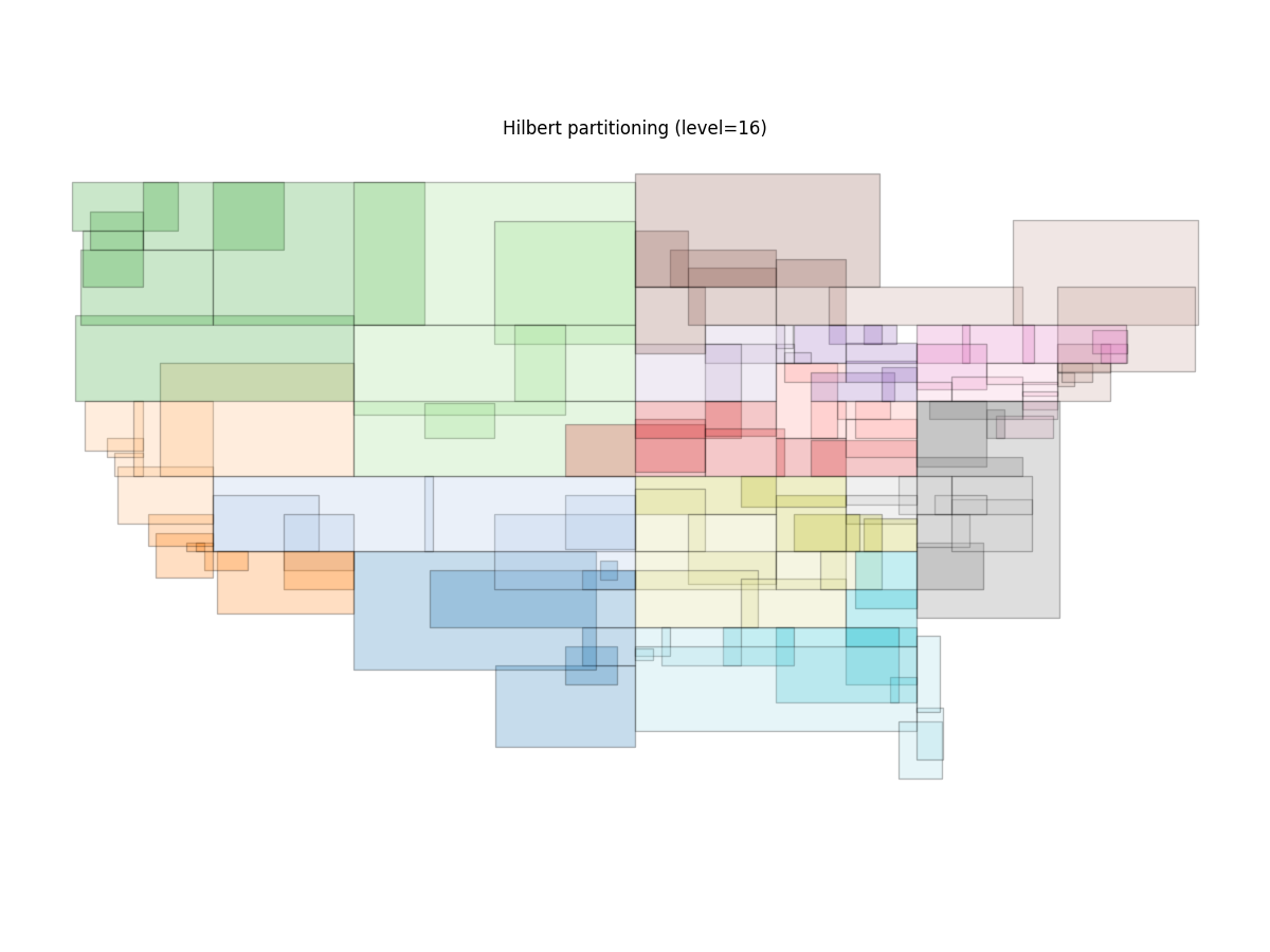
Now that they’re shuffled, we can plot the resulting spatial partitions:
r = dask_geopandas.read_parquet("data/hilbert-16.parquet")
ax = r.spatial_partitions.plot(edgecolor="black", cmap="tab20", alpha=0.25, figsize=(12, 9))
ax.set_axis_off()
ax.set(title="Hilbert partitioning (level=16)")
The outline of the United States is visible, and the spatial partitions do a good (but not perfect) job of making mostly non-overlapping, spatially compact partitions.
which gives

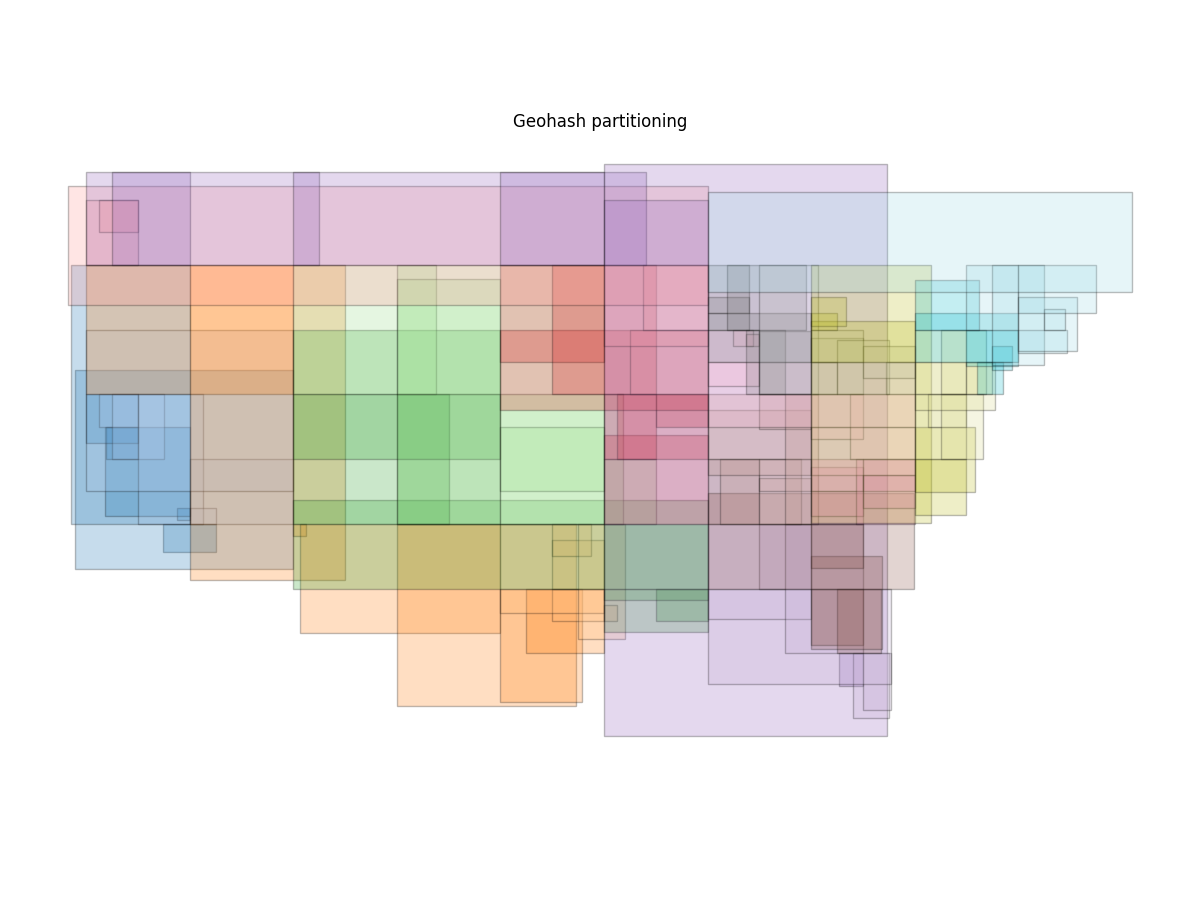
Here’s a similar plot for by="geohash"

And for by="morton"

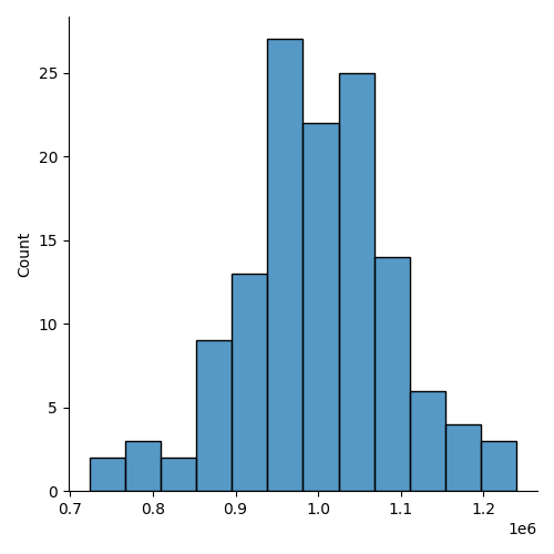
Each partition ends up with approximately 1,000,000 rows (our original chunk size). Here’s a histogram of the count per partition:
import seaborn as sns
counts = [fragment.count_rows() for fragment in pyarrow.parquet.ParquetDataset("data/hilbert-16.parquet/").fragments]

sns.displot(counts);

The discussion also mentions KD trees as potentially better way of doing the partitioning. I’ll look into that and will follow up if anything comes out of it.